Preprocessing Guide
Complete guide to building and applying preprocessing pipelines for Raman spectroscopy data.
Table of Contents
Overview
Why Preprocess?
Raman spectra often contain noise and artifacts that can interfere with analysis:
Common Issues:
📈 Baseline drift: Fluorescence background
📊 Noise: Random intensity fluctuations
📉 Intensity variations: Sample-to-sample differences
⚡ Cosmic rays: Sharp spikes from detector artifacts
Preprocessing Goals:
Remove or reduce unwanted signal components
Enhance relevant spectral features
Normalize intensity variations
Prepare data for analysis or ML
Preprocessing Philosophy
Best Practices:
✅ Less is more: Use minimal necessary steps
✅ Understand each step: Know what each method does
✅ Validate effects: Always preview before applying
✅ Document pipelines: Save and share for reproducibility
✅ Test order: Method sequence matters
Common Mistakes:
❌ Over-smoothing (loss of real features)
❌ Over-normalization (loss of quantitative information)
❌ Wrong method order (e.g., normalizing before baseline correction)
❌ Not validating on test set
❌ Using same parameters for all datasets
Pipeline Builder Interface
Main Layout
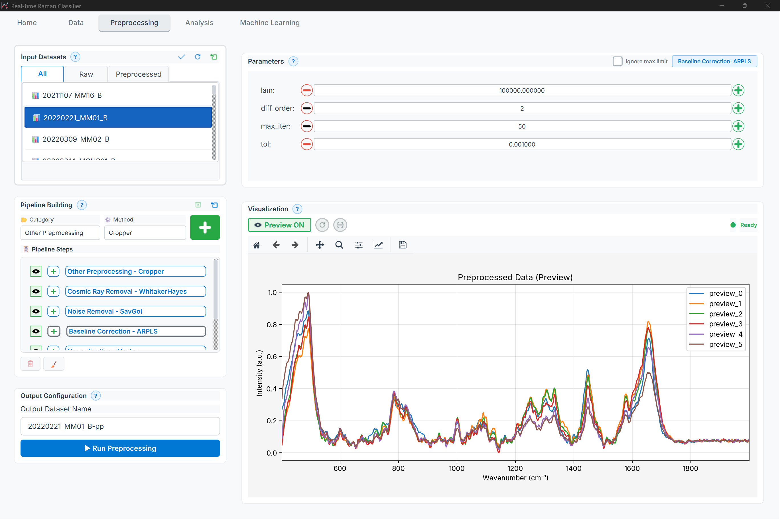
Figure: Preprocessing page showing method selector (left), parameter panel (center), and preview plot (right), with pipeline builder at the bottom
Note: The preprocessing page is divided into three main sections:
Left: Method selector with categories (Baseline, Smoothing, Normalization, etc.)
Center: Parameter configuration panel for the selected method
Right: Real-time preview showing before/after comparison
Bottom: Pipeline steps list with controls for each step (visibility, delete, reorder)
Components
1. Method Selector (Left Panel)
Browse 40+ preprocessing methods by category
Search by name or keyword
Hover for method description
2. Parameter Panel (Center)
Configure selected method
Real-time validation
Tooltips explain each parameter
Reset to defaults button
3. Preview Panel (Right)
Before/after comparison
Multiple spectra overlay
Zoom and pan
Statistics (SNR, baseline level)
4. Pipeline Steps (Bottom)
Ordered list of methods
Toggle enable/disable: ☑/☐
View parameters: 👁
Delete step: 🗑
Reorder: ⬆⬇
Drag to reorder
5. Action Buttons
Clear: Remove all steps
Save Pipeline: Export as JSON
Load Pipeline: Import from file
Apply to Dataset: Process all spectra
Method Categories
1. Baseline Correction
Purpose: Remove fluorescence background and baseline drift
AsLS (Asymmetric Least Squares)
Best for: General baseline correction
Parameters:
lambda(λ): Smoothness (1e2 - 1e9, default: 1e5)Lower → Flexible baseline
Higher → Smooth baseline
p: Asymmetry (0.001 - 0.1, default: 0.01)Lower → Fit peaks as baseline
Higher → Fit valleys as baseline
Example:
# Conservative: λ=1e5, p=0.01
# Aggressive: λ=1e7, p=0.001
AirPLS (Adaptive Iteratively Reweighted Penalized Least Squares)
Best for: Automatic baseline estimation
Parameters:
lambda: Smoothness (1e2 - 1e7, default: 1e5)porder: Penalty order (1, 2, default: 1)max_iter: Maximum iterations (10-100, default: 15)
When to use: Unknown baseline shape, automatic processing
Polynomial Baseline
Best for: Simple polynomial baseline
Parameters:
degree: Polynomial degree (1-10, default: 3)1 = linear
2 = quadratic
3-5 = most common
When to use: Smooth, predictable baseline
FABC (Fully Automatic Baseline Correction)
Best for: Completely automatic correction
Parameters:
window_length: Window size (100-500, default: 200)iterations: Number of iterations (1-20, default: 10)
When to use: No user tuning desired, batch processing
2. Smoothing and Denoising
Savitzky-Golay Filter
Best for: Noise reduction while preserving peaks
Parameters:
window_length: Window size (5-51, odd numbers, default: 11)Smaller → Less smoothing, more noise
Larger → More smoothing, peak broadening
polyorder: Polynomial order (2-5, default: 3)2 = quadratic
3 = cubic (recommended)
deriv: Derivative order (0-2, default: 0)0 = smoothing only
1 = first derivative
2 = second derivative
Example:
# Light smoothing: window=7, order=3
# Moderate: window=11, order=3
# Heavy: window=21, order=3
Gaussian Smoothing
Best for: Strong noise reduction
Parameters:
sigma: Standard deviation (0.5-5.0, default: 2.0)Lower → Less smoothing
Higher → More smoothing
When to use: Very noisy data, when peak shape preservation is less critical
Moving Average
Best for: Simple, uniform smoothing
Parameters:
window_size: Window size (3-21, default: 5)
When to use: Quick smoothing, preliminary exploration
Median Filter
Best for: Removing spike noise (cosmic rays)
Parameters:
window_size: Window size (3-11, odd numbers, default: 5)
When to use: Detector artifacts, cosmic ray spikes
3. Normalization
Vector Normalization (L2 Norm)
Best for: Intensity variations, general use
Formula: Divide each spectrum by its L2 norm
normalized = spectrum / sqrt(sum(spectrum^2))
When to use:
Remove intensity differences
Classification tasks
Most common choice
Min-Max Normalization
Best for: Scaling to fixed range [0, 1]
Formula:
normalized = (spectrum - min) / (max - min)
When to use:
Visualization
Neural networks
When you need bounded values
Area Normalization
Best for: Concentration normalization
Formula: Divide by area under curve
normalized = spectrum / sum(abs(spectrum))
When to use:
Comparing relative peak heights
Eliminating concentration effects
SNV (Standard Normal Variate)
Best for: Scattering correction
Formula:
snv = (spectrum - mean) / std
When to use:
Solid samples with scattering
Removing multiplicative effects
MSC (Multiplicative Scatter Correction)
Best for: Light scattering correction
Requirements: Reference spectrum (mean of all spectra)
When to use:
Diffuse reflectance spectroscopy
Particle size effects
4. Derivatives
First Derivative (Savitzky-Golay)
Best for: Baseline removal, peak resolution
Effect:
Removes baseline
Enhances peak differences
Converts peaks to positive/negative transitions
Parameters: Same as Savitzky-Golay filter + deriv=1
When to use:
Alternative to baseline correction
Improve peak separation
Chemometric analysis
Second Derivative
Best for: Peak sharpening, overlapping peaks
Effect:
Further sharpens peaks
Converts peaks to negative dips
Enhances fine structure
Parameters: Same as Savitzky-Golay filter + deriv=2
When to use:
Overlapping peak resolution
Peak identification
Advanced spectroscopic analysis
Warning: Amplifies noise significantly
5. Advanced Methods
Convolutional Denoising Autoencoder (CDAE)
Best for: Deep learning-based denoising
Requirements:
GPU recommended
Training data with clean/noisy pairs
PyTorch installed
Parameters:
model_path: Path to trained modelbatch_size: Processing batch size (8-64, default: 32)
When to use:
Complex noise patterns
After training on your specific data type
Wavelet Transform
Best for: Multi-resolution denoising
Parameters:
wavelet: Wavelet type (‘db4’, ‘sym8’, default: ‘db4’)level: Decomposition level (1-10, default: 4)threshold: Threshold method (‘soft’, ‘hard’, default: ‘soft’)
When to use:
Non-stationary noise
Multi-scale features
Peak Ratio Feature Engineering
Best for: Creating ratio features
Parameters:
peak1_range: [start, end] wavenumber for peak 1peak2_range: [start, end] wavenumber for peak 2
Output: New feature = Peak1 / Peak2
When to use:
Known biomarker ratios
Reducing dimensionality
Creating interpretable features
Building a Pipeline
Step-by-Step Guide
Example Task: Preprocess blood plasma Raman spectra for classification
Step 1: Start with Raw Data
Visualize:
Import spectra
Plot overlay of all spectra
Identify issues:
High baseline? → Need baseline correction
Noisy? → Need smoothing
Varying intensities? → Need normalization
Step 2: Add Baseline Correction
Choose Method:
# For fluorescence background:
AsLS (λ=1e5, p=0.01)

# For automatic:
AirPLS (λ=1e5)
Add to Pipeline:
Select “AsLS” from Baseline category
Set λ=1e5, p=0.01
Click [Preview] → Check effect
Adjust parameters if needed
Click [Add to Pipeline]
Preview Tips:
Overlay before/after
Check multiple representative spectra
Ensure peaks are not removed
Baseline should be flat near zero
Step 3: Add Smoothing (Optional)
When needed: If spectra still noisy after baseline correction
# Moderate smoothing:
Savitzky-Golay (window=11, polyorder=3, deriv=0)
Add to Pipeline:
Select “Savitzky-Golay”
Set window=11, polyorder=3
Preview and adjust
Add to pipeline
Warning: Don’t over-smooth!
Check peak widths
Compare to raw data
Ensure real features remain
Step 4: Add Normalization
Why last?:
Baseline correction first removes offsets
Smoothing reduces noise
Normalization as final step for intensity correction
# Most common:
Vector Normalization (L2)
Add to Pipeline:
Select “Vector Normalization”
No parameters needed
Preview
Add to pipeline
Final Pipeline:
1. AsLS Baseline (λ=1e5, p=0.01)
2. Savitzky-Golay (window=11, order=3)
3. Vector Normalization
Step 5: Validate Pipeline
Check on Representative Spectra:
Click each step’s 👁 (eye) to see effect
Toggle steps on/off to compare
Verify on different groups
Check edge cases (weak signal, high noise)
Quality Metrics:
SNR improvement
Peak preservation
Baseline flatness
Consistency across spectra
Step 6: Save and Apply
Save Pipeline:
Click [Save Pipeline]
Name:
blood_plasma_standard.jsonAdd description
Save to pipeline library
Apply to Dataset:
Select input data
Click [Apply to Dataset]
Progress bar shows processing
Processed spectra saved automatically
Common Pipelines
1. Standard Pipeline (General Purpose)
Pipeline: standard_preprocessing
1. AsLS Baseline (λ=1e5, p=0.01)
2. Savitzky-Golay Smoothing (window=11, order=3)
3. Vector Normalization

Use Case: General Raman spectroscopy, classification tasks
Pros: Robust, widely applicable, minimal parameter tuning
Cons: May not be optimal for specific cases
2. Minimal Pipeline (Low Noise Data)
Pipeline: minimal_preprocessing
1. Polynomial Baseline (degree=3)
2. Vector Normalization

Use Case: High-quality spectra, minimal noise
Pros: Fast, preserves maximum information
Cons: Not suitable for noisy or complex baseline
3. Aggressive Denoising (High Noise Data)
Pipeline: heavy_denoising
1. Median Filter (window=5)  # Remove spikes
2. AirPLS Baseline (λ=1e6)
3. Gaussian Smoothing (σ=2.0)
4. SNV Normalization

Use Case: Low signal-to-noise ratio, cosmic rays
Pros: Maximum noise reduction
Cons: Risk of over-smoothing, loss of fine features
4. Derivative-Based Pipeline
Pipeline: derivative_based
1. AsLS Baseline (λ=1e5, p=0.01)
2. Savitzky-Golay 1st Derivative (window=11, order=3, deriv=1)
3. Vector Normalization

Use Case: Baseline drift issues, overlapping peaks
Pros: Removes baseline, enhances peak differences
Cons: Amplifies noise, requires good smoothing
5. Chemometric Pipeline (Quantitative Analysis)
Pipeline: chemometric
1. AsLS Baseline (λ=1e6, p=0.001)
2. MSC (Multiplicative Scatter Correction)
3. Savitzky-Golay Smoothing (window=9, order=3)
4. Area Normalization

Use Case: Quantitative analysis, concentration prediction
Pros: Corrects scattering, preserves peak ratios
Cons: Requires reference spectrum for MSC
6. Deep Learning Preprocessing
Pipeline: deep_learning_prep
1. Median Filter (window=3)  # Remove outliers
2. AsLS Baseline (λ=1e5, p=0.01)
3. Min-Max Normalization [0, 1]

Use Case: Neural network input
Pros: Bounded values, simple normalization
Cons: May need data augmentation
Advanced Tips
Parameter Optimization
Grid Search for AsLS:
# Test combinations:
lambda_values = [1e3, 1e4, 1e5, 1e6, 1e7]
p_values = [0.001, 0.01, 0.1]

# For each combination:
# 1. Apply preprocessing
# 2. Run classification
# 3. Select best performing parameters
Optimization Tools:
Use ML page → Hyperparameter Optimization
Include preprocessing parameters
Cross-validate on training set only
Method Order Guidelines
General Rules:
Spike removal first: Median filter
Baseline correction next: AsLS, AirPLS, etc.
Smoothing: Savitzky-Golay, Gaussian
Derivatives (if used): After smoothing
Normalization last: Vector, SNV, etc.
Why this order?:
Spikes corrupt baseline estimation
Baseline affects normalization
Smoothing should be on baseline-corrected data
Normalization as final intensity correction
Computational Efficiency
For large datasets (>1000 spectra):
Disable real-time preview during building
Use batch processing: Process in chunks
Optimize parameters on subset first
Save pipelines for reuse
Consider GPU acceleration for deep learning methods
Validation Strategy
Split-Sample Validation:
1. Split data: 80% train, 20% test
2. Build pipeline on training set only
3. Apply same pipeline to test set
4. Evaluate on both sets
5. Ensure no overfitting to training data
Cross-Validation:
1. Use K-fold CV on training set
2. Apply same pipeline to each fold
3. Average performance across folds
4. Final test on held-out test set
Troubleshooting
Problem: Peaks Disappear After Preprocessing
Causes:
Over-smoothing
Aggressive baseline correction
Second derivative without smoothing
Solutions:
Reduce Savitzky-Golay window size
Lower AsLS lambda parameter
Skip derivative methods
Validate on known peaks
Problem: Baseline Still Present
Causes:
Insufficient lambda in AsLS
Wrong asymmetry parameter
Polynomial degree too low
Solutions:
Increase λ from 1e5 to 1e6 or 1e7
Adjust p parameter (try 0.001 for higher baseline)
Use higher polynomial degree or different method
Try AirPLS for automatic correction
Problem: Spectra Look Too Smooth
Causes:
Window size too large
Multiple smoothing steps
Gaussian sigma too high
Solutions:
Reduce window size
Remove redundant smoothing steps
Compare to raw data visually
Check if real peaks are lost
Problem: Pipeline Slow to Apply
Causes:
Large dataset
Computationally expensive methods (CDAE, wavelet)
Real-time preview enabled
Solutions:
Disable preview during application
Process in batches
Use faster methods (polynomial instead of AsLS)
Enable parallel processing in settings
Problem: Inconsistent Results
Causes:
Different preprocessing for train/test
Parameter randomness (if applicable)
Data leakage (normalizing before splitting)
Solutions:
Save and apply same pipeline to all data
Split data BEFORE preprocessing
Document exact pipeline used
Version control pipeline files
See Also
Analysis Methods Reference - Detailed method documentation
Data Import Guide - Prepare data for preprocessing
Analysis Guide - Next step after preprocessing
Best Practices - Preprocessing recommendations
Next: Analysis Guide →